Introduction to Bayesian Optimization for Medium Components

Introduction

Across all industries, continuous efforts are being made to improve productivity through material reviews, model refinement, and workflow improvements. In particular, for complex black-box systems whose underlying mechanisms are not well understood, finding optimal conditions can require significant time and cost. Biological systems are a prime example — even with the advances of modern biology, it remains difficult to accurately predict “how will cells behave if we add this environmental factor or medium component?” (though for model organisms, we can make somewhat better predictions).

Given these challenges, conducting experiments in the bio field is not only difficult but also expensive, making it impractical to collect massive datasets and test every possible condition exhaustively. For this reason, “knowledge-based optimization” relying on expert experience and intuition has been the mainstream approach. However, as biomanufacturing becomes increasingly sophisticated, the limitations of human expertise alone are becoming apparent, and the growing complexity of parameters makes straightforward optimization elusive.

As a result, the need to “achieve maximum results with as few experiments as possible” is rapidly growing.

This is where Bayesian optimization has attracted attention. It is already being actively used in fields such as materials informatics, and its effectiveness has been well demonstrated.

That said, adoption in the bio field is still in its early stages, with few reference cases and resources available. Moreover, since many bio researchers involved in medium optimization are not familiar with computer science, many may wonder, “Bayesian optimization? What’s that?”

In this article, we use a function that simulates cell behavior in response to medium component concentrations to explain the Bayesian optimization approach and the results it can produce. In practice, batch Bayesian optimization — which proposes multiple conditions at once — is the mainstream approach, but for clarity, we first present an example of sequential optimization, where conditions are updated one at a time. We then illustrate the expected results and explore the potential for applications in the bio field.

Creating a Function that Reproduces Cell Behavior

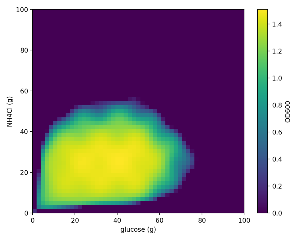
We described cells as a “black box” earlier, and indeed cells are a quintessential example of a black-box function. For instance, let us define the glucose amount as x g (carbon source) and NH₄Cl as y g (nitrogen source). Cell growth (OD₆₀₀) can then be expressed as f(x, y). In other words, cell proliferation can be treated as “a value output in response to inputs x and y.”

In this article, to keep the explanation simple, we define a two-dimensional function with glucose amount as x and nitrogen source NH₄Cl as y that exhibits certain behavior (we affectionately call it “Cell-kun”). For those with experimental experience, it should be easy to imagine: increasing medium components does not simply result in proportionally greater growth. In reality, complex interactions between components give rise to diverse growth patterns.

Here, we created a function f(x, y) that reflects this concept. Cell-kun based on this function exhibits the following behavior (the figure below shows the true distribution — if we knew this in advance, there would be no need for optimization).

In Bayesian optimization, we begin by acquiring a small number of initial experimental data points before starting the search. In this case, we simulated culturing “Cell-kun” under the following conditions as the initial experiment.

• x = Glucose amount (g)
• y = NH₄Cl amount (g)

The experimental conditions (x[g], y[g]) are the following 5 combinations:

(5.0 g, 5.0 g), (5.0 g, 95.0 g), (95.0 g, 5.0 g), (95.0 g, 95.0 g), (50.0 g, 50.0 g)

From these results, Cell-kun exhibited the following culture behavior.

Glucose (g)	NH₄Cl (g)	OD₆₀₀
5.0	5.0	0.761678
5.0	95.0	0.874593
95.0	5.0	0.879424
95.0	95.0	0.902424
50.0	50.0	1.079207

The following scripts can be executed from this link.

First, install the required packages for the analysis.

!pip -q install imageio openpyxl scikit-optimize

We load this data as a DataFrame for use in Python.

import pandas as pd
from io import StringIO

csv_text = """Glucose (g),NH4Cl (g),0D600
5.0,5.0,1.079207
5.0,95.0,0.000000
95.0,5.0,0.000000
95.0,95.0,0.000000
50.0,50.0,0.510030
"""

# String CSV → DataFrame
df_raw = pd.read_csv(StringIO(csv_text))

# Standardize column names: x=glucose, y=NH4Cl, od=OD600
seed_df = df_raw.rename(columns={"Glucose (g)": "x", "NH4Cl (g)": "y", "0D600": "od"})

# Verify
seed_df

The loaded result is displayed as follows.

　x　　　y　　　od
0  5.0   5.0   1.079207
1  5.0   95.0  0.000000
2  95.0  5.0   0.000000
3  95.0  95.0  0.000000
4  50.0  50.0  0.510030

Next, we prepare the model for Bayesian optimization.

from od_objective_2d import ODObjective2D, BOUNDS2D
from skopt import Optimizer
from skopt.space import Real
import numpy as np

# Generate the objective function (Cell-kun)
obj = ODObjective2D()

# Define the search range (lower/upper bounds for x=glucose, y=NH4Cl)
space = [Real(BOUNDS2D["x"][0], BOUNDS2D["x"][1], name="x"),
         Real(BOUNDS2D["y"][0], BOUNDS2D["y"][1], name="y")]

# Create the Bayesian optimizer
opt = Optimizer(
    dimensions=space,
    base_estimator="GP",  # Use Gaussian Process as the internal surrogate model
    acq_func="EI",  # Acquisition function: Expected Improvement determines "which point to measure next"
    random_state=7
)

best_od = -np.inf
best_xy = (None, None)
rows = []
for i, r in seed_df.reset_index(drop=True).iterrows():
    xi, yi, odi = float(r["x"]), float(r["y"]), float(r["od"])
    opt.tell([xi, yi], -odi)
    if odi > best_od:
        best_od, best_xy = odi, (xi, yi)
    rows.append({"iter": i+1, "phase": "seed", "x": xi, "y": yi, "od": odi,
                 "best_so_far": best_od, "best_x": best_xy[0], "best_y": best_xy[1]})

ODObjective2D is the function representing Cell-kun’s behavior (outputting OD values). In this case as well, we use this model to evaluate the results of conditions proposed by the model. Note that in actual practice, since the function is not available, you would skip this process and simply input measured values.

Optimizer(...): Creates the Bayesian optimizer.

• base_estimator="GP": Uses Gaussian Process as the internal surrogate model.
• acq_func="EI": Uses Expected Improvement to determine “which point to measure next.”

With this, the preparation is complete! Let’s actually run it as follows.

n_iters = 20  # Total number of experiments

print("\n=== Starting Bayesian Optimization (Experimental Design → Experiment → Model Query) ===")
for t in range(1, n_iters+1):
    # 1) ask: Propose one point to measure next
    x_next, y_next = opt.ask()
    print(f"[BO iter {t}] Proposed point: Glucose={x_next:.3f}, NH4Cl={y_next:.3f}")

    # 2) Experiment (demo: calling the function; replace with actual measurements in practice)
    od_measured = float(obj(x_next, y_next))
    print(f"            Measured OD= {od_measured:.6f}")

    # 3) tell: Pass the new observation to the BO
    opt.tell([x_next, y_next], -od_measured)

    # 4) Check for best update
    improved = ""
    if od_measured > best_od:
        best_od, best_xy = od_measured, (x_next, y_next)
        improved = "  ← ★ New best!"

    rows.append({
        "iter": len(rows)+1, "phase": "bo",
        "x": x_next, "y": y_next, "od": od_measured,
        "best_so_far": best_od, "best_x": best_xy[0], "best_y": best_xy[1],
    })
    print(f"            Current best = {best_od:.6f} @ {best_xy}{improved}")

n_iters corresponds to how many times the process of model-based condition proposal and evaluation is performed. Since this is an in silico experiment, we can run it infinitely, but in practice this value is constrained by the budget.

This produces the following output.

=== Starting Bayesian Optimization (Experimental Design → Experiment → Model Query) ===
[BO iter 1] Proposed point: Glucose=22.734, NH4Cl=31.897
            Measured OD= 1.421598
            Current best = 1.421598 @ (22.733907982646524, 31.89722257734033)  ← ★ New best!
[BO iter 2] Proposed point: Glucose=97.822, NH4Cl=45.558
            Measured OD= 0.000000
            Current best = 1.421598 @ (22.733907982646524, 31.89722257734033)
[BO iter 3] Proposed point: Glucose=30.801, NH4Cl=26.387
            Measured OD= 1.464924
            Current best = 1.464924 @ (30.80127651877394, 26.387083903789872)  ← ★ New best!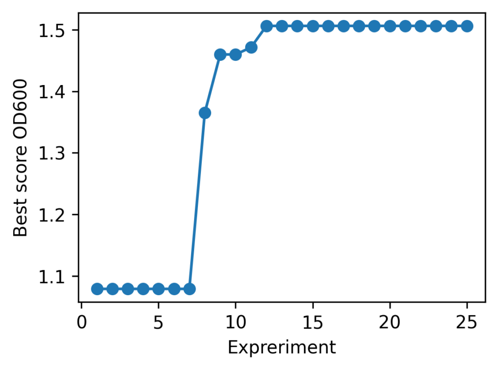

With Cell-kun’s behavior in this case, a total of 12 experiments including the initial ones yielded:

best_OD₆₀₀	best_glucose (g)	best_NH₄Cl (g)
1.505	41.280	26.775

It appears that Cell-kun has quite a high glucose requirement.

As demonstrated, Bayesian optimization — which may seem daunting at first — can be applied to practical use with just a bit of coding. We hope this article provides some value for your medium optimization efforts.

In this article, we used a simple optimization example with two parameters for clarity, but most real-world problems involve higher dimensions. Furthermore, multi-objective optimization that simultaneously considers not only growth but also product yield and quality is often required.

Our company provides a high-performance optimization system called “Epistra Accelerate.” We can accommodate individual use cases, so if you have questions about more advanced optimization or applying it to real data, please feel free to contact us.

In this example, one experimental condition was proposed and evaluated per round. However, in general, it is more common to compare multiple conditions in parallel during each round. This pattern is known as batch Bayesian optimization. In the next article, we will tackle medium optimization for Cell-kun using batch Bayesian optimization.

Next article: Introduction to Bayesian Optimization for Medium Components (Batch Optimization)

---

Execution Environment

The programs described on this page have been tested using Google Colab. To ensure reproducibility, the Python version and major library versions are listed below.

Last verified: November 10, 2025

Python Version

Python 3.10.12 (Google Colab default)

Library Versions

Library	Version
dataclasses	0.6
imageio	2.37.0
matplotlib	3.10.0
numpy	2.0.2
openpyxl	3.1.5
pandas	2.2.2
scikit-optimize	0.10.2