Introduction to Bayesian Optimization for Medium Components (Batch Optimization)

Introduction

In the previous article, we introduced an approach using sequential optimization, where one condition is generated per round and the model is updated each time. However, in real-world experiments, it is common to test multiple conditions in parallel within a single round. In this article, we present an implementation example of such “batch optimization.”

See the previous article on sequential optimization here

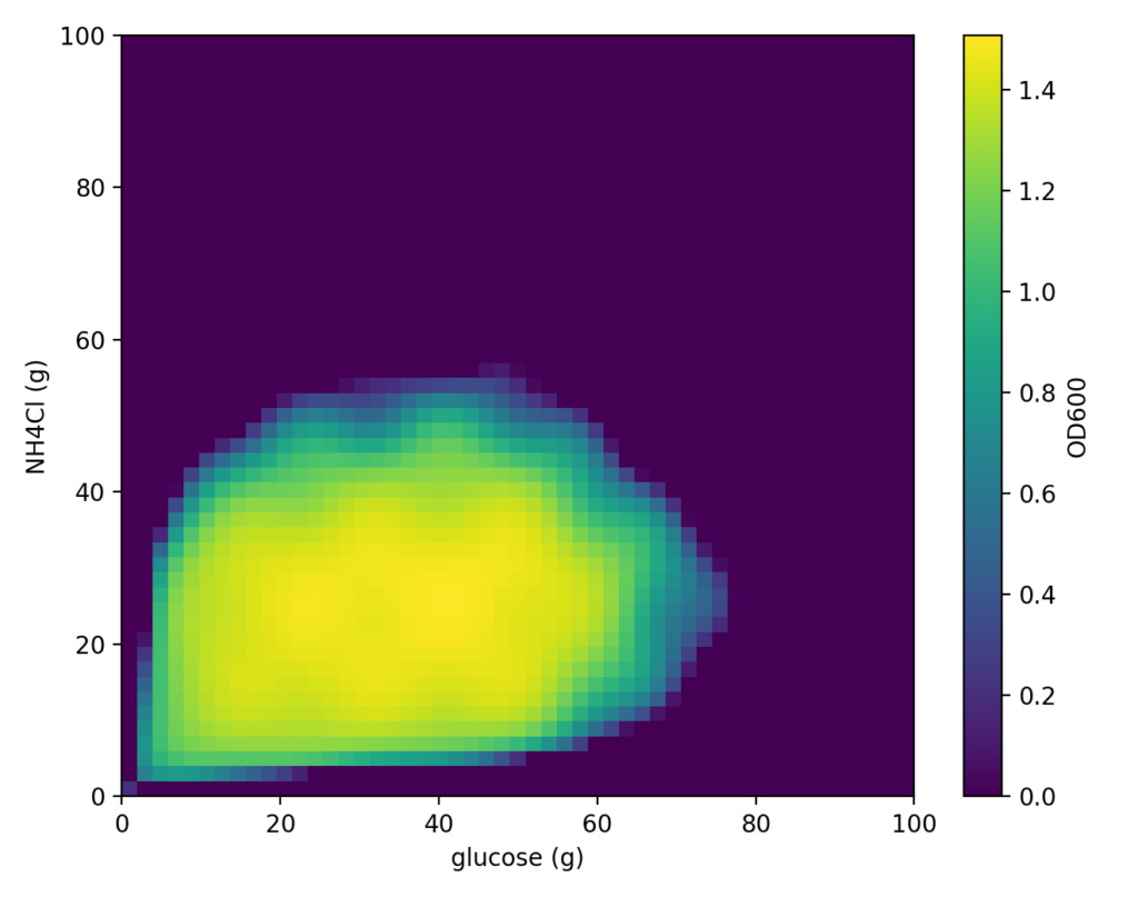
For this cell simulation as well, we will search for optimal medium conditions using the “Cell-kun” function introduced last time. As a reminder, this “Cell-kun” function is a two-dimensional function that exhibits certain behavior with glucose amount as x and nitrogen source NH₄Cl as y. The distribution is shown below.

Continuing from the previous article, we set the following measured values as initial data.

Glucose (g)	NH₄Cl (g)	OD₆₀₀
5.0	5.0	0.761678
5.0	95.0	0.874593
95.0	5.0	0.879424
95.0	95.0	0.902424
50.0	50.0	1.079207

The following scripts can be executed from this link.

First, install the required packages for the analysis.

!pip -q install imageio openpyxl scikit-optimize

Next, load the initial data into a Python DataFrame.

import pandas as pd
from io import StringIO

csv_text = """Glucose (g),NH4Cl (g),0D600
5.0,5.0,1.079207
5.0,95.0,0.000000
95.0,5.0,0.000000
95.0,95.0,0.000000
50.0,50.0,0.510030
"""

# String CSV → DataFrame
df_raw = pd.read_csv(StringIO(csv_text))

# Standardize column names: x=glucose, y=NH4Cl, od=OD600
seed_df = df_raw.rename(columns={"Glucose (g)": "x", "NH4Cl (g)": "y", "0D600": "od"})

# Verify
seed_df

Next, we prepare the model for Bayesian optimization.

from od_objective_2d import ODObjective2D, BOUNDS2D
from skopt import Optimizer
from skopt.space import Real
import numpy as np

# Generate the objective function (Cell-kun)
obj = ODObjective2D()

# Define the search range (lower/upper bounds for x=glucose, y=NH4Cl)
space = [Real(BOUNDS2D["x"][0], BOUNDS2D["x"][1], name="x"),
         Real(BOUNDS2D["y"][0], BOUNDS2D["y"][1], name="y")]

# Create the Bayesian optimizer
opt = Optimizer(
    dimensions=space,
    base_estimator="GP",  # Use Gaussian Process as the internal surrogate model
    acq_func="EI",  # Acquisition function: Expected Improvement determines "which point to measure next"
    random_state=7
)

best_od = -np.inf
best_xy = (None, None)
rows = []
for i, r in seed_df.reset_index(drop=True).iterrows():
    xi, yi, odi = float(r["x"]), float(r["y"]), float(r["od"])
    opt.tell([xi, yi], -odi)
    if odi > best_od:
        best_od, best_xy = odi, (xi, yi)
    rows.append({"iter": i+1, "phase": "seed", "x": xi, "y": yi, "od": odi,
                 "best_so_far": best_od, "best_x": best_xy[0], "best_y": best_xy[1]})

Here,

ODObjective2D is a function that simulates the behavior of “Cell-kun.” In actual experiments, you would skip this part and input measured values instead.

Running Batch Optimization

This is where the implementation diverges from the previous article.

n_rounds = 10      # Number of rounds (each round proposes batch_size conditions)
batch_size = 2     # Number of conditions proposed per round

print("\n=== Starting Bayesian Optimization (Batch Proposals) ===")
for r in range(1, n_rounds + 1):
    # 1) ask: Propose batch_size points to measure next, all at once
    X_next = opt.ask(n_points=batch_size, strategy="cl_min")
    print(f"[BO round {r}] Proposed points:")
    for j, (x_next, y_next) in enumerate(X_next, start=1):
        print(f"  cond{j}: Glucose={x_next:.3f}, NH4Cl={y_next:.3f}")

    # 2) Experiment (demo: using objective function; replace with actual OD measurements in practice)
    od_list = [float(obj(xn, yn)) for (xn, yn) in X_next]
    for j, odm in enumerate(od_list, start=1):
        print(f"    → cond{j} measured OD= {odm:.6f}")

    # 3) tell: Pass all results to the BO model at once
    opt.tell(X_next, [-od for od in od_list])

    # 4) Check for best update & append to log
    for j, ((xn, yn), odm) in enumerate(zip(X_next, od_list), start=1):
        improved = ""
        if odm > best_od:
            best_od, best_xy = odm, (xn, yn)
            improved = "  ← ★ New best!"

        rows.append({
            "iter": len(rows) + 1,
            "phase": "bo",
            "round": r,
            "cond_in_round": j,
            "x": xn,
            "y": yn,
            "od": odm,
            "best_so_far": best_od,
            "best_x": best_xy[0],
            "best_y": best_xy[1],
        })
        print(f"    cond{j}: current best = {best_od:.6f} @ {best_xy}{improved}")

# Check the best point found internally by skopt (result of minimizing -OD)
best_idx = int(np.argmin(opt.yi))
skopt_best_xy = tuple(opt.Xi[best_idx])
skopt_best_od = -opt.yi[best_idx]

print("\n=== Final Summary ===")
print(f"Log best: OD={best_od:.6f} @ {best_xy}")
print(f"skopt best: OD={skopt_best_od:.6f} @ {skopt_best_xy}")

The optimization was run with the following settings:

n_rounds = 10      # Number of rounds (each round proposes batch_size conditions)
batch_size = 2     # Number of conditions proposed per round

Two conditions are proposed per round, each evaluated and fed back into the model. The optimal conditions obtained are as follows:

=== Starting Bayesian Optimization (Batch Proposals) ===
[BO round 1] Proposed points:
  cond1: Glucose=98.874, NH4Cl=85.862
  cond2: Glucose=98.328, NH4Cl=10.249
    → cond1 measured OD= 0.000000
    → cond2 measured OD= 0.000000
    cond1: current best = 1.079207 @ (5.0, 5.0)
    cond2: current best = 1.079207 @ (5.0, 5.0)
[BO round 2] Proposed points:
  cond1: Glucose=57.559, NH4Cl=98.794
  cond2: Glucose=64.765, NH4Cl=55.086
    → cond1 measured OD= 0.000000
    → cond2 measured OD= 0.000000
    cond1: current best = 1.079207 @ (5.0, 5.0)
    cond2: current best = 1.079207 @ (5.0, 5.0)
[BO round 3] Proposed points:
  cond1: Glucose=35.263, NH4Cl=53.854
  cond2: Glucose=24.801, NH4Cl=9.849
    → cond1 measured OD= 0.266920
    → cond2 measured OD= 1.370388
    cond1: current best = 1.079207 @ (5.0, 5.0)
    cond2: current best = 1.370388 @ (24.800715628900235, 9.848637049589822)  ← ★ New best!

 ~omitted~

[BO round 10] Proposed points:
  cond1: Glucose=29.950, NH4Cl=29.855
  cond2: Glucose=50.098, NH4Cl=33.738
    → cond1 measured OD= 1.472082
    → cond2 measured OD= 1.455068
    cond1: current best = 1.472082 @ (29.949798427708167, 29.85455402401584)  ← ★ New best!
    cond2: current best = 1.472082 @ (29.949798427708167, 29.85455402401584)

The progress of batch optimization is summarized in the line chart below.

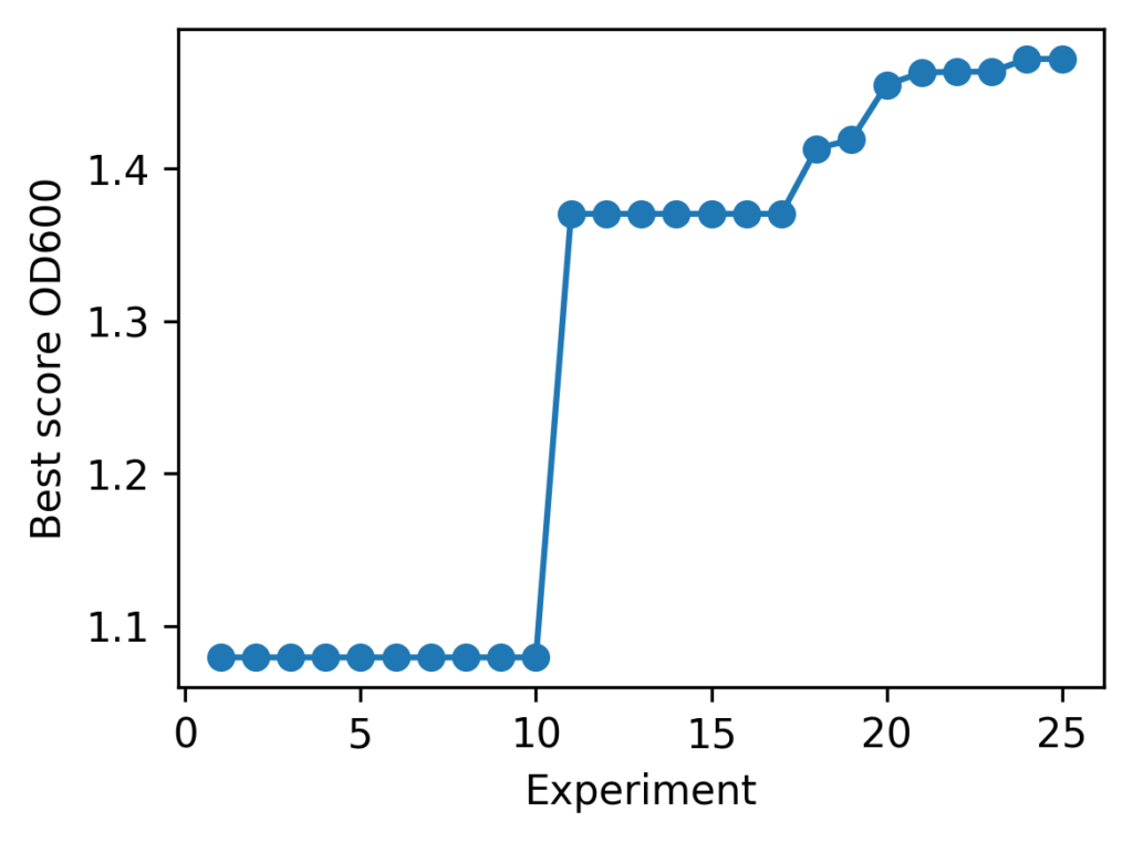
As a result, the following medium composition was identified as the optimal solution:

best_od	best_glucose (g)	best_NH₄Cl (g)
1.472082	29.949798427708167	29.85455402401584

Comparison with Sequential Optimization

So far, we have presented the batch optimization implementation and its results. How does batch optimization differ from sequential optimization, where the model is updated one condition at a time? Comparing the optimization results for the same “Cell-kun” makes the difference clear. Below are the results of sequential optimization from the previous article and batch optimization from this article.

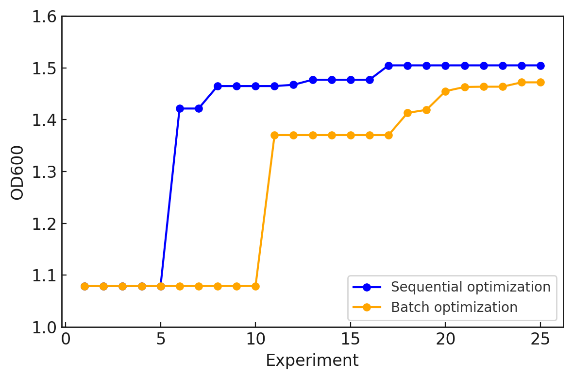
We can see that sequential optimization converges faster and achieves slightly better performance. In sequential optimization, the model can be updated after each experiment, so search efficiency is generally higher. On the other hand, batch optimization enables parallel experiments, but since the model is updated less frequently, search efficiency is lower. However, in real research, situations such as “a single culture run takes one month” are common, making sequential optimization impractical. When considering experimental efficiency, batch optimization becomes more useful in practice. In other words, there is a trade-off between search accuracy and experimental efficiency.

The choice of which to prioritize depends on the research environment. In this article, we introduced a batch optimization implementation and compared it with sequential optimization to highlight their respective characteristics. We hope that this series of simulations mimicking cell behavior has helped you envision applications in the life sciences field.

---

Execution Environment

The programs described on this page have been tested using Google Colab. To ensure reproducibility, the Python version and major library versions are listed below.

Last verified: November 10, 2025

Python Version

Python 3.10.12 (Google Colab default)

Library Versions

Library	Version
dataclasses	0.6
imageio	2.37.0
matplotlib	3.10.0
numpy	2.0.2
openpyxl	3.1.5
pandas	2.2.2
scikit-optimize	0.10.2